Minimum Color Path Problems

Let us revisit the shortest path problem in graphs. We are given an edge weighted graph, a source and a destination vertex and , respectively, and we want to find a path between and having the minimum weight. The problem can be solved in polynomial time using any standard shortest path algorithm. Now, consider a slight variant of this problem, where the weights are dependent in the sense that if you pay a cost for an edge, you do not need to pay the cost for some other edges. One can think that the underlying graph is a road network, where every edge is a road, and the weights are the tolls that we need to pay to go along the edges. Then two edges might correspond to the same road and thus if you already have paid the toll for using the road, you do not need to pay the toll for the same road again. The standard way to formulate this problem is to consider a graph, where a set of colors is associated with every vertex, and you want to find a path s.t. the size of the union of the sets corresponding to the vertices along the path is minimized. This problem is called the Minimum Color Path (MCP) problem (also Minimum Constraint Violation Problem). In the following example a-b-c is an optimal path having 4 colors.

The problem in general graphs can be shown to be hard using a reduction from Set Cover. If you are wondering about applications, let me give you two concrete ones.

1. Minimum Obstacle Removal: Given a collection of geometric objects in the plane, and two points s,t, find a simple curve between s and t that intersects the interior of the minimum number of objects. The problem appears naturally in robot path planning.

We can construct a graph from the input instance in the following way. Consider a vertex placed on each cell of the input arrangement. For each vertex, associate the set of objects corresponding to its cell. Join two vertices with an edge if the two cells are adjacent. Basically the graph is the dual graph of the planar input arrangement, and hence planar. Then an optimal obstacle removal path is a path in this graph that has the minimum size union of the sets corresponding to its vertices.

2. Minimum Barrier Resilience:  Given a collection of wireless sensor regions, represented by disks in the plane, two points and , find the minimum number of  regions an intruder at needs to hack to get access at . Basically is protected by a shield of networks. One can model this problem as the MCP problem.

An approximation for a restricted version of MCP: The assumption is that there is an optimal path, where each color appears at most times. The algorithm is the following. Forget about the colors and replace each set by its size. Find minimum weight path in the graph. The minimum weight path must have weight OPT, where OPT is the optimal number of colors needed. Thus the returned path uses at most OPT colors leads to an approximation. This is a universal trick to get approximation for this problem. Let us discuss about some previous work in the geometric setting.

Unit squares: 2 approximation.

Unit disks: 3 approximation

Minimum constraint removalGeneral squares/disks: No sublinear approximation is known.

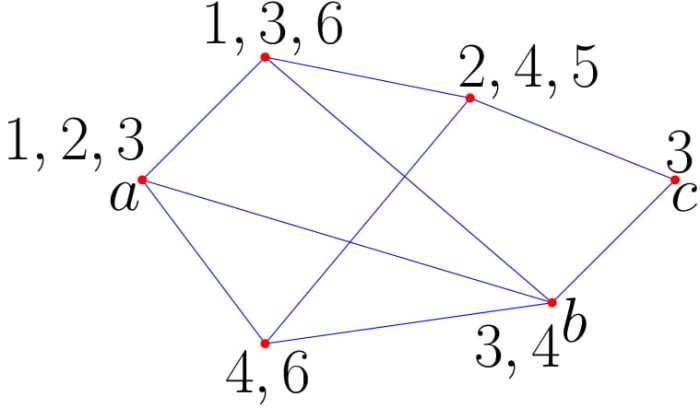
In the following, we discuss an algorithm for MCP. Let me just take a step back and discuss a Dynamic programming based algorithm for standard shortest path – Floyd-Warshall. For any path, call a vertex exposed if it is one of the two end vertices. Otherwise, it is hidden. Note that any s-t path will have a fixed cost, which is the sum of the weights of s and t. Thus we always consider only the hidden vertex costs for a path. At last we can add the fixed cost to find the total cost of the path. The DP formulation is as follows, where $S_k$ is the set corresponding to the vertex k.

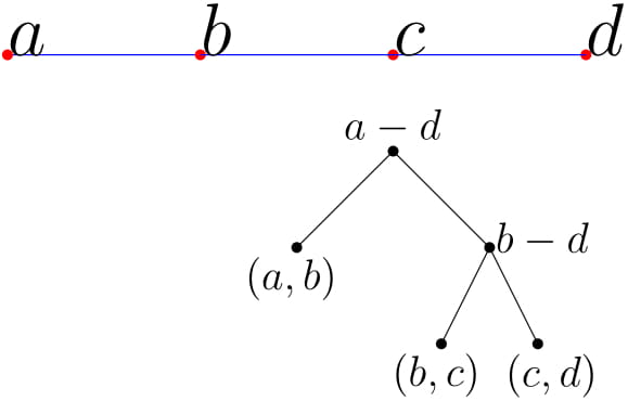
One way to analyze this algorithm is the following. We show the existence of a witness tree (binary) which emulates the computation of the algorithm. The root is corresponding to an optimal s-t path. Each leaf is corresponding to an edge. For each internal node, merge the paths of the two children to find a path for the node. Here is an example.

So, this algorithm surely does not work for our case, as it might charge the same color a lot of times. But, note that to address the multiple counting issue, we can come up with some discounting scheme, where we try to avoid the multiple counting. Let’s consider the following discounting scheme. We charge a color while merging if it appears in k, but not in i or j. The modified DP formulation is as follows.

$latex d_t(i,j)=\min\{\min_k d_{t-1}(i,k)+d_{t-1}(k,j)+|S_k\setminus \{S_i\cup S_j\}|,d_{t-1}(i,j)\}$

Let us take a simple example to see how does this scheme work.

Here the graph is a path, and contains two colors a and b.

Thus the discounting scheme can detect almost half of the double countings. To improve the bound let us consider another strategy. The discounts would be more accurate if we keep more exposed vertices. So, we index by two paths now instead of just one path. And, you always do not charge a color if it appears in one of the exposed vertices. The algorithm is called 2-path algorithm (in general Multipath algorithm). For our previous example the hidden cost is thus zero as shown in the following derivation of the optimal path.

 

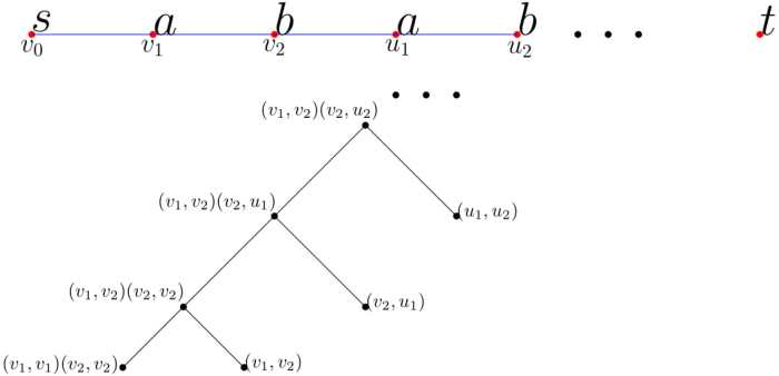
Here all the colors are appearing  in one of the exposed vertices. Thus if k is |OPT|, then k-path algorithm is sufficient to find the optimal cost. But runtime depends exponentially on k.

Analysis of the Multipath Algorithm: While computing the path in bottom up manner we see that for two vertices and  sharing a color, the color will not be charged for both ,  if either of them appears as an exposed vertex at the step when the other vertex becomes hidden. To make sure that what we can do is add the leaf to the derivation tree. This process is logically similar to adding an arc between and on a fixed optimal path to identify the conflict. But it is not guaranteed if only t indexes are sufficient to derive an optimal path using those leaves. Here one can use the property that only bounded number of colors appear in an optimal path. Thus there we need lesser number of arcs. Note that each such arc saves a double counting. Thus even if we can have at least constant fraction of such arcs, we can identify a constant fraction of the double countings and that leads to a constant factor approximation. For Unit disks one can actually get a 2 approximation using this scheme.

See this paper for more details.